Consumer demand-driven historical data are characterized to a large extent by seasonal patterns (consumer habits: economics) and trends (consumer demographics: population growth and migration). For the sample data, this can be readily shown using the ANOVA: Two Factor without Replication option in Excel Data Analysis Add-in. The data shown in the spreadsheet have an unusual value in January 2016. identified in the a previous post in my website blog; when adjusted it has a significant effect on the variation impacting seasonality (consumer habit) while reducing unknown variation.

Demand forecasting in today’s disrupted consumer demand-driven supply chain environment has become extremely challenging. For situations when – in pre new-normal times – demand occurs sporadically, the challenge becomes even greater. Intermittent data (also known as sporadic demand) comes about when a product experiences periods of zero demand. This has become more common during the pandemic supply chain, especially in the retail industry. The Levenbach L-Skill score, introduced here, is applicable in a ‘regular’ as well as intermittent lead-time demand forecasting process.

First Takeaway: Embrace change & chance by first improving data quality through exploratory data analysis (EDA). It is an essential preliminary step in improving forecasting performance.

A New Objective Approach to Lead-time Demand Forecasting Performance Evaluation

When assessing forecasting performance, standard measures of forecast accuracy can be distorted by a lack of robustness in normality (Gausianity) assumptions even in a ‘regular’ forecasting environment. In many situations, just a single outlier or a few unusual values in the underlying numbers making up the accuracy measure can make the result unrepresentative and misleading. The arithmetic mean, as a typical value representing an accuracy measure can ordinarily only be trusted as representative or typical when data are normally distributed (Gaussian iid). The arithmetic mean becomes a very poor measure of central tendency even with slightly non-Gaussian data (unusual values) or sprinkled with a few outliers.  This is not widely recognized among demand planners and commonly ignored in practice. Its impact on forecasting best practices needs to be more widely recognized among planners, managers and forecasting practitioners in supply chain organizations.

Imagine a situation in which you need to hit a target on a dartboard with twelve darts, each one representing a month of the year. Your darts may end up in a tight spot within three rings from the center. Your partner throws twelve darts striking within the first ring but somewhat scattered around the center of the dartboard. Who is the more effective dart thrower in this competition? It turns out that it depends not only how far the darts land from the center but also on the precision of the dart thrower.

In several recent posts on my LinkedIn Profile and this Delphus website blog, I laid out an information-theoretic approach to lead-time demand forecasting performance evaluation for both intermittent and regular demand. In the spreadsheet example, the twelve months starting September, 2016 were used as a holdout sample or training data set for forecasting with three methods: (1) the previous year’s twelve-month actuals (Year-1) as a benchmark forecast of the holdout data, (2) a trend/seasonal exponential smoothing model ETS(A,A,M), and (3) a twelve-month average of the previous year (MAVG-12). The twelve-month point forecasts over the fixed horizon of the holdout sample are called the Forecast Profile (FP). Previous results show that the three Mean Absolute Percentage Errors (MAPE) are about the same around 50%, not great but probably typical, especially at a SKU-location level.

We now want to examine the information-theoretic formulation in more detail in order to derive a skill score so that we can use it to assess the effectiveness of the forecasting process or the forecaster in terms of how much the method, model or forecaster contributed to the benefit of the overall forecasting process.

Creating an Alphabet Profile

For a given Forecast Profile FP, the Forecast Alphabet Profile FAP is a set of positive weights whose total sums to one. Thus, a Forecast Alphabet Profile is a set of m positive fractions FAP = [f₁ f₂, . . f_m] where each element f_i is defined by dividing each point forecast by the sum or Total of the forecasts over the horizon (here m = 12). This will give us fractions whose sum equals one.

Likewise, the Actual Alphabet Profile is AAP = [a₁, a₂, . . . a_m], where a_i is defined by dividing the Leadtime Total into each actual value and a Forecast Alphabet Profile FAP = [f₁ f₂, . . f_m], where f_i is defined by dividing the Leadtime Total into each forecast value. When you code a forecast profile FP into the corresponding alphabet profile FAP, you can see that the forecast pattern does not change.

For profile forecasting performance, we use a measure of information H, which has a number of interpretations in different application areas like climatology and machine learning. The information about the actual alphabet profile (AAP) is H(AAP) and the information about a forecast alphabet profile (FAP) is H(FAP), both entropy measures. There is also a measure of information H(a|f) about the FAP given we have the AAP information.

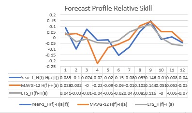
A Forecast Profile Error is defined by FPE _* a_i Ln a_i minus f_i Ln f_i, where Ln denotes the natural logarithm. Then summing the profile errors gives us the Forecast Profile Miss = H(f) – H(a):

The Accuracy D(a|f) of a forecast profile is defined as the Kullback-Leibler divergence measure D(a|f) = H(a|f) – H(a), where H(a|f) = – Sum (a_i Ln f_i ).

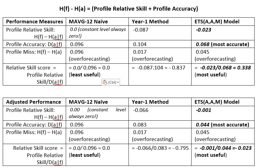
If we rewrite D(a|f) = [H(a|f) – H(f)] + [H(f) – H(a)], it results in a decomposition of profile accuracy into two components, namely the (1) Forecast Profile Miss = H(f) – H(a) and (2) a Relative Skill measure: H(f) – H(a|f), , the negative of the first bracketed term in the expression for D(a|f).

Another way of looking at this is using Forecast Profile Miss = Profile Accuracy + Relative Skill. In words, this means that accurately hitting the bullseye requires both skill at aiming and considering how far from the bullseye the darts strike the board.

The Relative Skill is in absolute value greater than zero, but does not include zero. The smaller, in absolute value, the better the Relative Skill and the more useful the method becomes. Remember, “All models are wrong, some are useful“, according the George Box. When a FAP is constant, as with the Croston methods, SES and MAVG-12 point forecasts, the Relative Skill = 0, meaning that with those methods, obtaining an (unbiased) Profile Bias of zero is clearly not possible. Hence, these methods are not useful for lead-time forecasting over fixed horizons. The M-competitions are examples of lead-time forecasting over fixed horizons.

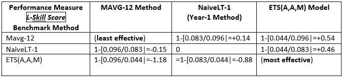
For using forecasts on an ongoing basis, it might be useful to create an accuracy Skill score , defined by 1 – [D(a|f) / D(a|f*)] , where f* is a benchmark forecast, like the Year-1 Method, which is commonly used in practice. For lead-time forecasting applications, I call this the Levenbach L-Skill score. By tracking the L-Skill scores of the methods, models and judgmental overrides used in the forecasting process over time with, we have a means of tracking the effectiveness of forecasting methods.

Final Takeaway

In the context of a multistep-ahead forecasting process with a fixed horizon, we can assess the contribution of a method, model or forecaster in the performance of a forecasting process with the L-Skill score. In theory, statistical forecasting models are designed to be unbiased, but that theoretical consideration may not be valid in practice, particularly for ‘fixed horizon’ lead-time demand forecasting. Moreover, multiple one-step ahead forecasts have little practical value in lead-time demand forecasting as the lead-time is the ‘frozen’ time window in which operational changes can usually not be made.

Try it out on some of your own data and see for yourself what biases and performance issues you have in your lead-time demand forecasts and give me some of your comments in the meantime. I think it depends on the context and application, so be as specific as you can. Let me know if you can share your data and findings.

Hans Levenbach, PhD is Executive Director, CPDF Professional Development Training and Certification Programs. Dr. Hans is the author of a new book (Change&Chance Embraced) on Demand Forecasting in the Supply Chain and created and conducts hands-on Professional Development Workshops on Demand Forecasting and Planning for multi-national supply chain companies worldwide. Hans is a Past President, Treasurer and former member of the Board of Directors of the International Institute of Forecasters.

Embracing Change and Chance. The examination of an forecasting process would not be complete until we consider the performance of the forecasting process or forecasters. This new Levenbach L-skill score measure of performance is included in my latest revision of the paperback available on Amazon (https://amzn.to/2HTAU3l).