When was the last time you saw moving average forecasts being used for forecasting sales, inventory, production or Supply Chain training and certification programs? Hopefully, not within the past two decades, because the methodology is incredibly outdated. Here is why.

In the past, when computing was expensive and data storage very limited, a forecaster did not have much recourse except to calculate with very limited computing power. That was my early experience as a Forecast Manager in a corporate environment. A Moving Average forecast is easy to implement using only arithmetic. So, why are we still using a method that results in multi-step (lead-time) forecasts that are always level, no matter what the historical data patterns are? Let me show you why.

Here is a sample of four time series (IST01, IST02, IST03, and IST04, each with three years (36 months) of real-world historical data. The context of the data is not important here because a Moving Average forecast does not make use of any additional information about the data. The four monthly series have been normalized so that the overall average in each series is the same (=985).

In a Moving Average forecast, what matters is the smoothing window (say 12, because the data are monthly and could be seasonal). Applying the Moving Average method, the forecasts for periods 36, 37, 38, etc. are equal to the average of the latest twelve values in the history (periods 25 – 36). In this case, we get 1045 (for IST01), 879 (for IST02), 1273 (for IST03), and 1052 (for IST04). This may seem reasonable, but not credible, if you are expecting level line forecasts without any further data analysis.

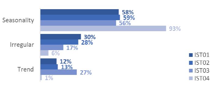
With modern computing power and ample storage for large data sets, it is a smarter practice to always take some exploratory data analysis steps prior to forecast modeling. Here, with consumer-driven demand, we recognize seasonality (i.e. consumer/customer habits), trend (i.e. consumer/customer demographics) and an uncertainty factor (i.e. all other variation not explained by trend and seasonality) as the dominant variation. To get a handle on demand variability, we decompose the variation into three components using a data analysis Add-in available in Excel (Two-way ANOVA without Replication). For the four series, this can be summarized graphically with pie charts.

More than 50% of the variation can be attributed to seasonality (either multiplicative or additive, yet to be determined), with dominant seasonality in IST04. The trend variation does not stand out, what is an exception, as actual consumer/customer-driven demand profiles are generally not level. Added to that, we observe that the uncertainty factor (labelled irregular) is not small, except in IST04. The uncertainty factor has a direct bearing on the width and skewness of the prediction intervals (error bounds) derived by creating forecasts with statistical models. High uncertainty thus means we should forecast broad and varying prediction intervals, and therefore this pre-modeling analysis suggests that the Moving Average forecasting method should not be considered. Generally, consumer/customer-driven demand forecasts are not level, so the method could very well be relegated to the dustbin.

The next step is to run the models. We already know that trend and seasonality are the primary drivers of demand in supply chain environments. To be credible and effective, we should utilize model algorithms with trend/seasonal forecast profiles. The ErrorTrendSeasonal (ETS) models have been accessible since the mid-1990s in a unified State-Space Forecasting methodology (including both exponential smoothing and ARIMA models). They have the flexibility to do the job. You can find them online in open source R-libraries and as a license free Excel Add-in on www.peerforecaster.com. The ETS models can distinguish between additive and multiplicative patterns in the trend, seasonal and error components.

To complete the modeling phase of the forecasting process, we can display the results in predictive visualization charts depicting the history (36 periods), the trend/seasonal forecast profile (12 periods) and the prediction limits (uncertainty bounds). The four “optimum” forecast profiles obtained by ETS (ErrorTrendSeasonality) modeling.

The corresponding Moving Average forecast profiles have been included, so that we see where we would have been led, had we applied this method instead of ETS statistical models. The charts show the ETS profiles fluctuating as expected, reproducing seasonality in a credible way, and also presenting a range, embodying the uncertainty we have about the future of each data set. The Moving Average results, on the other hand, extend resolutely into the future, with its typical steady profile, with zero response to trend, seasonality and uncertainty, drawing a completely unlikely pattern for real supply chain demand profiles, so the method could very well be relegated to the dustbin.

There are a number of time series forecasting textbooks on the market explaining State Space Forecasting, including my own book Chance&Chance Embraced: Achieving Agility with Smarter Forecasting in the Supply Chain and the CPDF® Smarter Forecasting and Planning Workshop Manual on Amazon.com

A Final Note: Uncertainty is a Certain Factor

A Moving Average forecast is a method, not a statistical modeling approach. With a statistical modeling approach, it is possible to provide prediction limits (error bounds) to characterize the uncertainty factor. This is not possible with a moving average method. And forecasts are tools that we use to navigate through (certain) uncertainty.

Hans Levenbach, PhD is Executive Director, CPDF Training and Certification Programs. Dr. Hans created and conducts hands-on Professional Development Workshops on Demand Forecasting for multi-national supply chain companies worldwide. Hans is a Past President, Treasurer and former member of the Board of Directors of the International Institute of Forecasters. He is group manager of the LinkedIn groups (1) Demand Forecaster Training and Certification, Blended Learning, Predictive Visualization, and (2) New Product Forecasting and Innovation Planning, Cognitive Modeling, Predictive Visualization.

I invite you to join these groups and share your thoughts and experiences.