As a follow-up to my previous article on smarter intermittent demand forecasting, I will now provide an algorithmic modeling approach for setting suitable safety stock levels without normality (Gaussian) assumptions. Forecasting intermittent demand occurs in practice, when

• modeling product mix based on future patterns of demand at the item and store level
• selecting the most appropriate inventory control policy based on type of stocked item
• setting safety stock levels for SKUs at multiple locations

Intermittent demand or ID (also known as sporadic demand) comes about when a product experiences several periods of zero demand. Often in these situations, when demand occurs it is small, and sometimes highly variable in size. The level of safety stock depends on the service level you select, on the replenishment lead time and on the reliability of the forecast.

Before making any modeling assumptions, we should first examine the characteristics of the underlying demand history in an exploratory data analysis. The spreadsheet table shows spare parts inventory data for Part #0174. We are looking for a lead-time (=3 periods) forecast and a level of safety stock to be used in an inventory management investigation.

Step 1. Explore the nature of the interdemand intervals and its relation to the distribution of non-zero demand sizes over a specified lead-time. See my previous article on the SIB modeling approach for this.

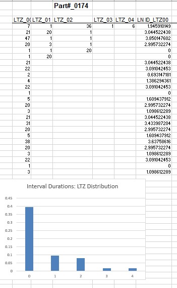
Examining the intermittent data with SIB models differs fundamentally from a Croston-based method in that this new (and smarter) approach does not assume that intervals and demand sizes are independent. The evidence of the dependence on interval durations for demand size can be shown by examining the frequency distribution of ‘lag time’ durations. I will define” Lag Time” Zero­­ interval LTZ as the interval duration preceding a demand size.

A Structured Inference Base (SIB) Model for Lead Time Demand

Step 2. For lead-time demand safety stock level selection, a location scale measurement error model can be viewed as a black box model. The Leadtime demand size LD in an intermittent or regular demand history can be represented as the output of a SIB location-scale measurement model LD = β + σ ɛ, in which β and σ are unknown parameters and the input ɛ is a measurement error with a known or assumed distribution. The SIB approach is algorithmic, data-driven, in contrast to a conventional data generating model with normality assumptions. The measurement model for Leadtime Demand LD is LD = β + σ ɛ is known as a location scale measurement model because of its structure. 

The text you add here will only be seen by users with visual disabilities. It will not be visible on the article itself.CancelSave

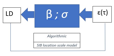
In a practical application, we may need to represent LD by a multivariate measurement error representing each lead-time for the demand, as typically the lead-time is an average and is not fixed, but for now we will assume ɛ = ɛ (τ) will depend on a typical lead time, represented by a single constant τ. The black box model shows that the output LD results from a translation and scaling of an input measurement error ɛ(τ), in which a conditioned measurement error distribution depends on a fixed, typical lead-time τ.

Keeping in mind the pervasive presence of outliers and non-normal (non-Gaussian) variation in the real-world intermittent demand forecasting environment, I will shy away from the usual normal distribution assumptions, which I refer to as the “gaussian arithmetic” mindset; it tends to view the arithmetic mean, standard deviation and CV as credible summary measures in these applications. Rather, I will assume a flexible family of distributions for ɛ(τ), known as the exponential family. It contains many familiar distributions including the normal (Gaussian) distribution, as well as ones with thicker tails and skewness. There are also some technical reasons for selecting the exponential family, besides its flexibility.

What Can Be Learned About the Measurement Process Given THIS Black Box Model and the Data?

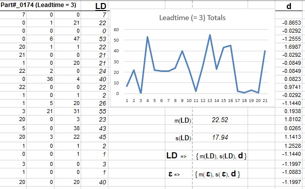
Step 3. We can analyze the model for lead-time demand size LD as follows. In practice, we have multiple measurements LD = {LD 1, LD 2, LD 3., . . ., LD n} of observed Leadtime demand over a time horizon, as shown in the spreadsheet example below. The output of the location-scale measurement model is

LD1 = β + σɛ1(τ) 

LD2 = β + σɛ2(τ) 

LD3 = β + σɛ3(τ)

LDn = β + σɛ(τ) 

where ɛ (τ) = {ɛ1(τ), ɛ2(τ), ɛ3(τ), . . . ɛn(τ)} are now n realizations of measurement errors from an assumed distribution in the exponential family with typical lead time τ.

Step 4. What information can we uncover about the black box process? Like a detective, we would discover that, based on the data, there is information revealed now about the unknown, but realized measurement errors ɛ(τ). This revelation will guide us to the next important SIB modeling step, namely a decomposition of the measurement error distribution into two components: (1) a marginal distribution for the observed components with fixed (τ) and (2) a conditional distribution (based on the observed components) for the remaining unknown measurement error distribution. So, what are these observed components of the error distribution that we uncover?

The insight or essential information is gleaned from the structure of the black box and the recorded output data. If we select a location metric m(.) (e.g. min LDi , arithmetic mean) and a scale metric s(.) (e.g. the range, standard deviation, or a first difference |LD2 – LD1 )|, we can make a calculation which gives observable information about the measurement process. Then the black box process shows (with substitution and some simple manipulations) and leaving out the (τ) notation, that

That is,

LD = m(LD) + s(LD) d and ɛ = m (ɛ) + s(ɛ) d

Step 4. Now, the n left-hand sides of the equations named d(LD) is equal to d(ɛ), which is the right-hand side of the equations. In the spreadsheet example for the 21 Leadtime demand values for Part #0174, d = d(LD) = d(ɛ) is shown in a column on the right side of the spreadsheet. For convenience of interpretation, we have selected the sample mean for the location metric m(.) and the sample standard deviation as the scale metric s(.).

To convince yourself that the above equations work, think of the scale metric s(.) as the sum of the squared LD observations or as a sample standard deviation, then as you multiply each LD value by the same constant c, the metric s(.) is scaled by the same constant c. In other words, s(c x) = c s(x), where c is a constant and x = (x1, x2, x3, … x n) are the data or observations. As it turns out, the choice of the metric is not important in the SIB inferential procedure, as long as s(.) has the above property. For m(.) we require that m(x + a) = a + m(x). Some metrics may turn out to be easier to process in the computations than others depending on the choice of the error distribution. These algorithms can be readily implemented in today’s computing environment, but that was not the case four decades ago. With a normal (Gaussian) error distribution assumption, there is a closed form solution (i.e. solvable in a mathematical analysis).

The distributions can be evaluated by computations that are doable on the computer; the formulae can be found in D.A.S. Fraser’s 1979 book Inference and Linear Models, Chapter 2, and in peer reviewed journal articles dealing with statistical inference and likelihood methods. (Statistical inference refers to the theory, methods, and practice of forming judgments about the parameters of a population and the reliability of statistical relationships).

Step 5. The important conditioning step is somewhat like what a gambler can do knowing the odds in a black jack game. The gambler can make calculations and should base inferences from what is observed in the dealt cards. We do the same thing here with our “inference game” box.

The useful information we can derive from this analysis is a decomposition of the measurement error distribution. This is the decomposition we have been alluding to for the error distribution:  ɛ ==> {m (ɛ), s(ɛ), d}, where the first two components are unknown scalars and the remaining component d is a known array of numbers, computable from the data. In the spreadsheet example for Part# 0174), m(LD) = 22.52 ands(LD) = 17.94. When using these formulas, recognize that the bold face items are arrays of numbers (vectors) and the normal type face symbols are numbers (scalars).

The Reduced Model

Taking these two equations for LD and ɛ, and substituting in the model equations ɛ = (LD – β)/ σ, we see that

m (ɛ) + s(ɛ) d = [m(LD) + s(LD) d – β]/ σ.

This reduces the unknown error components from n to 2. Knowing that d(ɛ) = d(LD), we have a reduced model for the two unobservable error components given by

s(ɛ) = s(LD)/ σ; for Part#0174 in the spreadsheet, we find that s(ɛ) = 17.94/ σ

m(ɛ) = [m(LD) – β]/ σ; for Part#0174 in the spreadsheet, we find that m (ɛ) = [22.52 – β]/ σ.

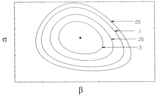
In the next, and final step, we use this to construct confidence intervals for the unknown parameters β and σ.

Step 6. The inferential analysis will yield a posterior distribution, conditional on d(ɛ) = d(LD, for the unknown parameters β and σ from which we can derive unique confidence bounds for β and σ and related likelihood inferences for τ. These confidence bounds will give us the service levels we require to set desired level of safety stock.

In short,

• No independence assumptions made on demand size and demand Interval distributions
• Create bootstrap samples from a SIB model for the underlying empirical distributions on an ongoing basis
• Determine posterior Lead-time demand distribution with MCMC sampling algorithms
• Determine upper tail percentiles of a lead-time demand distribution from family of exponential distributions for lead-time demands.

Hans Levenbach, PhD is Executive Director, CPDF Professional Development Training and Certification Programs. Dr. Hans created and conducts hands-on Professional Development Workshops on Demand Forecasting and Planning for multi-national supply chain companies worldwide. Hans is a Past President, Treasurer and former member of the Board of Directors of the International Institute of Forecasters. He is group manager of the LinkedIn groups (1) Demand Forecaster Training and Certification, Blended Learning, Predictive Visualization, and (2) New Product Forecasting and Innovation Planning, Cognitive Modeling, Predictive Visualization.