Forecasting intermittent demand occurs in practice, when 

• creating lead time demand forecasts for inventory planning.
• creating multiple forecasts of low volume items for a particular period in the future based on a rolling forecast horizon, as in an annual budget or production cycle.
• creating forecasts for multiple periods in an 18-month business planning horizon.

Intermittent Demand (ID also known as sporadic demand) comes about when a product experiences multiple periods of zero demand. Often in these situations, when demand occurs it is small, and sometimes highly variable in size.

Before making any modeling assumptions, we should first examine an application and the underlying historical data. Exploratory data analysis and forecast modeling are treated in my new book on demand forecasting principles and best practices, available in paperback and Kindle e-book for smartphone and tablet reading on Amazon.

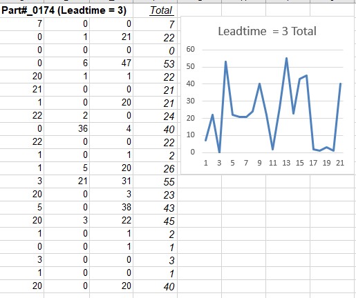
The rows in the spreadsheet table shows 63 historical values of spare parts inventory data for Part #0174. We are looking for a lead-time (= 3 periods) forecast to be used in an inventory application.

Step 1. Explore the nature of the interdemand intervals and the relation to the distribution of non-zero demand sizes over a specified lead-time.

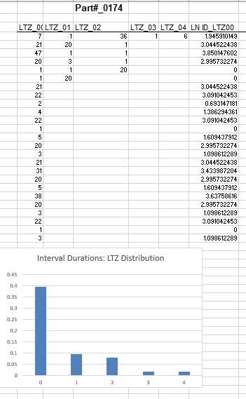
We first examine the relationship between intervals and demand sizes. As in my previous article, a ”Lag time” Zero­­ Interval LTI is defined as the interval duration preceding a demand size. The results are shown below. In this dataset there are five LZI interval durations. For example, the first LZI_03 interval has three zeros preceding the demand size 1. The next LZI_00 interval has no zeros preceding the demand size 21. The next one LZI_04 has four zeros followed by a demand size (- 6)and so on. A frequency distribution of the LZI intervals shows that contiguous demand sizes occur 25 out of the 63 occurrences (=40%), while LZI_03 and LZI_04 occur only once.

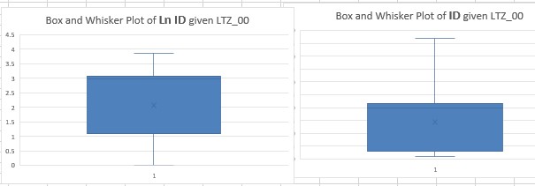
Examining the data in this way differs fundamentally from a Croston-based method in that this new and smarter approach, called the SIB model does not assume that intervals and demand sizes are independent. The evidence of dependence on interval duration is clearly evident in the LZI frequency distribution. It should also be clear from the two box and whisker plots that the log transformed data Ln ID is more symmetrical than the original ID data, which is good practice as it could more closely resemble normally distributed demand sizes.

A Structured Inference Base (SIB) Model for Forecasting Lead Time Demand

In a previous blog on SIB models for forecasting, I introduced measurement error models for forecasting intermittent demand sizes based on the dependence of an LZI interval distribution.

For lead-time demand forecasting applications below, a scale measurement error model can be viewed as a black box model. The Leadtime Demand size LD in an intermittent or regular demand history can be represented as the output of a location-scale measurement model LD = β + σ ɛ, in which β and σ are unknown parameters and the input ɛ is a measurement error with a known or assumed distribution. This equation can be rewritten as LD = σ (ø + ɛ), where ø = β /σ. This is known as a scale measurement error model LD = σ ɛ*, where ɛ* = ø + ɛ. It is a multiplicative measurement model with error ɛ*= ø + ɛ and scale parameter σ. We will call ø a shape constant for the ɛ* distribution. 

In a practical application, we may need to represent LD by a multivariate measurement error representing each lead-time for the demand, as typically the lead-time is an average and is not fixed, but for now we will assume ɛ*(τ) will depend on a typical lead time, represented by a single constant τ.

Keeping in mind the pervasive presence of outliers and non-normal (non-Gaussian) variation in the real-world intermittent demand forecasting environment, we will have to shy away from the normal distribution in what I refer to as the “gaussian arithmetic” mindset, which views the arithmetic mean, sample standard deviation and CV as credible summary measures in these situations. Rather, we will assume a flexible family of distributions for ɛ*, known as the exponential family. It contains many familiar distributions including the normal (Gaussian) distribution, as well as ones with thicker tails and skewness. There are also some technical reasons for selecting the exponential family, besides its flexibility.

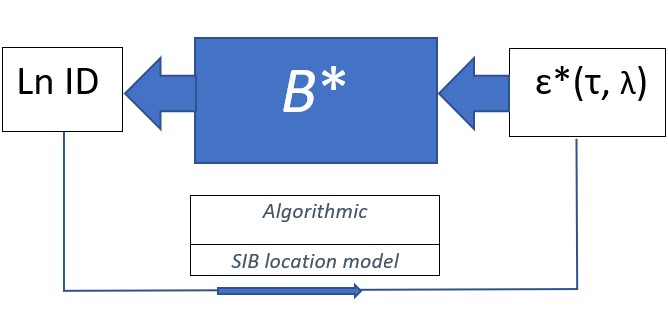
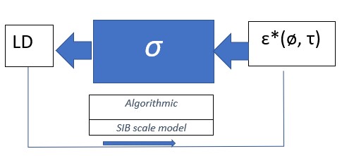
The SIB approach is algorithmic, data-driven, in contrast to a conventional data-model with normality assumptions. The measurement model for Leadtime Demand LD is LD = σ ɛ*. is known as a scale model because of its structure. What can be learned about the measurement process given THIS black box model and the data?

The black box model LD = σ ɛ*(τ, ø) shows that the output LD results from a scaling of an input measurement error ɛ*(τ, ø), scaled by a constant σ , in which a conditioned measurement error distribution depends on a fixed shape parameter ø and a typical lead-time τ.

Step 2. Starting with the SIB scale model, analyze the model for lead-time demand size LD.

In the spreadsheet example, we have multiple measurements LD = {LD 1, LD 2, LD 3., . . ., LD 21} of 21 observed leadtime demand sizes over a time horizon. The output of the scale measurement model is

LD1 = σɛ1*(τ, ø) 

LD2 = σɛ2*(τ, ø) 

LD3 = σɛ3*(τ, ø)

LD21 = σɛ21*(τ, ø) 

where ɛ *(τ, ø) = {ɛ1*(τ, ø), ɛ2*(τ, ø), ɛ3*(τ, ø), . . . ɛ21*(τ, ø)} are now 21 realizations of measurement errors from an assumed distribution with fixed shape constant ø and typical lead time τ in the exponential family.

The question now is what information can we uncover about the black box process? What we find may perhaps appear somewhat unfamiliar to those who have been through a statistics course on Inferential methods. If you could explore the innards of the black box like a detective, you would discover that, based on the data, there is information now about the unknown, but realized measurement errors ɛ*(τ, ø). This revelation will guide us to the next important step SIB modeling process, namely a decomposition of the measurement error distribution into two components: (1) a marginal distribution for the observed components with fixed (τ, ø) and (2) a conditional distribution (based on the observed components) for the remaining unknown measurement error distribution, which will not depend on (τ, ø). So, what are these observed components of the error distribution that we could expose?

The insight or essential information is gleaned from the structure of the black box and the recorded output data. If we select a scale metric like the range, standard deviation, or a first difference LD2 – LD1 for scale, we can make a calculation which gives observable information about the measurement process. Let’s call this scale metric s(LD). Then the black box process reveals (with substitution and some simple manipulations) and leaving out the (τ, ø) notation, that

LD1 / s(LD) = σɛ1 */ s(σɛ*)

 = σɛ1 */ σs(ɛ*)

 = ɛ1 */ s(ɛ*)

LD2 /s(LD) = ɛ2*/s(ɛ*)

LD3 /s(LD) = ɛ3*/s(ɛ*)

.

LD21 /s(LD) = ɛ21*/s(ɛ*)

Notice that the left-hand side of each equation can be calculated from the data, so the right-hand side is information about a realized measurement error ɛ*and its distribution.

What is known we can condition on, so we can derive a conditional distribution given the known error component and a marginal distribution for the known error component with fixed shape parameter ø and typical lead time τ. We do not need to go further into details at this time. This is doable, and can be found in D.A.S. Fraser’s 1979 book (p.20), and in peer reviewed journal articles. This is doable data science in today’s computing environment, but that was not the case four decades ago because it is computationally intensive, except when assuming an unrealistic normal distribution,

The important conditioning step is somewhat like what a gambler can do knowing the odds in a black jack game. The gambler can make calculations and should base inferences from what is observed in the dealt cards. We do the same thing here with our “inference game” box.

To convince yourself that the above equations work, think of the scale metric s(.) as the sum of the squared observations or sample standard deviation, then as you multiply each observation by the same constant c, the metric s(.) is scaled by the same constant c. In other words, s(c x) = cs (x), where c is a constant and x = (x1, x2, x3, … x n) are the data or observations. As it turns out, the choice of the metric is not important in the SIB inferential procedure, as long as s(.) has the above property. Some metrics may turn out to be easier to process in the computations than others depending on the choice of the error distribution.

The useful information we can derive from this analysis is a decomposition of the measurement error distribution. The analysis will yield a (conditional) posterior distribution for the unknown parameter σ from which we can derive unique confidence bounds for σ and related likelihood inferences for the (τ, ø) constants. This will give us the ability to specify safety stock numbers based on a prescribed stock out probability in an inventory forecasting and planning process, while embracing change and chance.

I will not dwell on the details here because, as data scientists you can compute using your own data. The location-scale measurement model and its generalizations were worked out over four decades ago by D.A.S. Fraser in his book Inference and Linear Models (1979), Chapter 2, and in a number of academic journal articles dealing with statistical inference and likelihood methods. (Statistical inference refers to the theory, methods, and practice of forming judgments about the parameters of a population and the reliability of statistical relationships.)

The scale measurement model is an application of a Structured Inference Base (SIB) approach that can be generalized to a wide range of applications. In a future article I will elaborate on the details of the SIB process for establishing safety stock for inventory planning and making inferences for the unknown constants in a spare parts inventory problem.